Introduction to Variational Autoencoders (VAEs): From Basics to Advanced Applications

Welcome to another comprehensive guide from TowardsCloud! Today, we’re diving into the fascinating world of Variational Autoencoders (VAEs) – a powerful type of deep learning model that’s revolutionizing how we generate and manipulate data across various domains.

What You’ll Learn in This Article

• The fundamental concepts behind autoencoders and VAEs
• How VAEs differ from traditional autoencoders
• Real-world applications across cloud providers
• Implementation considerations on AWS, GCP, and Azure
• Hands-on examples to deepen your understanding

🔍 Call to Action: Are you familiar with autoencoders already? If not, don’t worry! This guide starts from the basics and builds up gradually. If you’re already familiar, feel free to use the table of contents to jump to more advanced sections.

Understanding Autoencoders: The Foundation

Before we dive into VAEs, let’s establish a solid understanding of regular autoencoders. Think of an autoencoder like a photo compression tool – it takes your high-resolution vacation photos and compresses them to save space, then tries to reconstruct them when you want to view them again.

Real-World Analogy: The Art Student

Imagine an art student learning to paint landscapes. First, they observe a real landscape (input data) and mentally break it down into essential elements like composition, color palette, and lighting (encoding). The student’s mental representation is simplified compared to the actual landscape (latent space). Then, using this mental model, they recreate the landscape on canvas (decoding), trying to make it as close to the original as possible.

Component	Function	Real-world Analogy
Encoder	Compresses input data into a lower-dimensional representation	Taking notes during a lecture (condensing information)
Latent Space	The compressed representation of the data	Your concise notes containing key points
Decoder	Reconstructs the original data from the compressed representation	Using your notes to explain the lecture to someone else

💡 Call to Action: Think about compression algorithms you use every day – JPEG for images, MP3 for audio, ZIP for files. How might these relate to the autoencoder concept? Share your thoughts in the comments below!

From Autoencoders to Variational Autoencoders

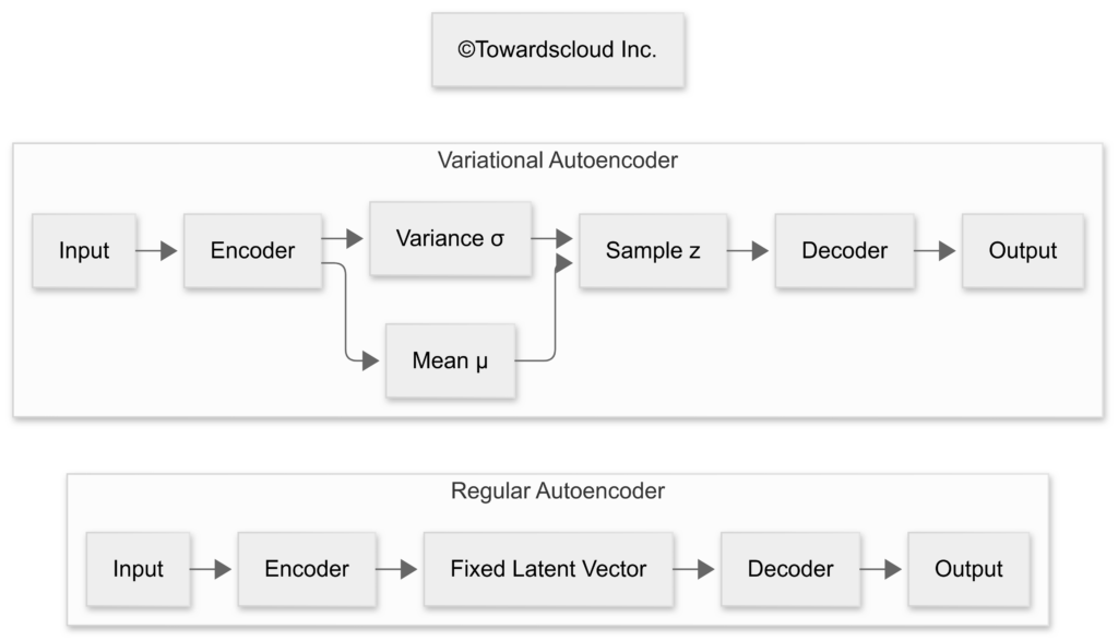
While autoencoders are powerful, they have limitations. Their latent space often contains “gaps” where generated data might look unrealistic. VAEs solve this problem by enforcing a continuous, structured latent space through probability distributions.

The VAE Difference: Adding Probability

Instead of encoding an input to a single point in latent space, a VAE encodes it as a probability distribution – typically a Gaussian (normal) distribution defined by a mean vector (μ) and a variance vector (σ²).

Real-World Analogy: The Recipe Book

Imagine you’re trying to recreate your grandmother’s famous chocolate chip cookies. A regular autoencoder would give you a single, fixed recipe. A VAE, however, would give you a range of possible measurements for each ingredient (e.g., between 1-1.25 cups of flour) and the probability of each measurement being correct. This flexibility allows you to generate multiple variations of cookies that all taste authentic.

Feature	Traditional Autoencoder	Variational Autoencoder
Latent Space	Discrete points	Continuous probability distributions
Output Generation	Deterministic	Probabilistic
Generation Capability	Limited	Can generate novel, realistic samples
Interpolation	May produce unrealistic results between samples	Smooth transitions between samples
Loss Function	Reconstruction loss only	Reconstruction loss + KL divergence term

The Mathematics Behind VAEs

Let’s break down the technical aspects of VAEs into understandable terms:

1. The Encoder: Mapping to Probability Distributions

The encoder in a VAE doesn’t output a direct latent representation. Instead, it outputs parameters of a probability distribution:

2. The Reparameterization Trick

One challenge with VAEs is how to backpropagate through a random sampling operation. The solution is the “reparameterization trick” – instead of sampling directly from the distribution, we sample from a standard normal distribution and then transform that sample.

3. The VAE Loss Function: Balancing Reconstruction and Regularization

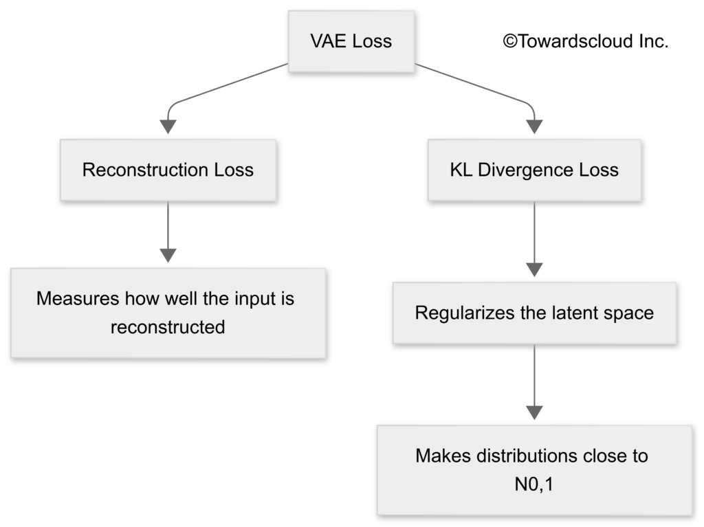
The VAE loss function has two components:

1. Reconstruction Loss: How well the decoder reconstructs the input (similar to regular autoencoders)
2. KL Divergence Loss: Forces the latent distributions to be close to a standard normal distribution

🧠 Call to Action: Can you think of why enforcing a standard normal distribution in the latent space might be beneficial? Hint: Think about generating new samples after training.

Real-World Applications of VAEs

VAEs have found applications across various domains. Let’s explore some of the most impactful ones:

1. Image Generation and Manipulation

VAEs can generate new, realistic images or modify existing ones by manipulating the latent space.

2. Anomaly Detection

By training a VAE on normal data, any input that produces a high reconstruction error can be flagged as an anomaly – useful for fraud detection, manufacturing quality control, and network security.

3. Drug Discovery

VAEs can generate new molecular structures with specific properties, accelerating the drug discovery process.

4. Content Recommendation

By learning latent representations of user preferences, VAEs can power sophisticated recommendation systems.

Industry	Application	Benefits
Healthcare	Medical image generation, Anomaly detection in scans, Drug discovery	Augmented datasets for training, Early disease detection, Faster drug development
Finance	Fraud detection, Risk modeling, Market simulation	Reduced fraud losses, More accurate risk assessment, Better trading strategies
Entertainment	Content recommendation, Music generation, Character design	Personalized user experience, Creative assistance, Reduced production costs
Manufacturing	Quality control, Predictive maintenance, Design optimization	Fewer defects, Reduced downtime, Improved products
Retail	Product recommendation, Inventory optimization, Customer behavior modeling	Increased sales, Optimized stock levels, Better customer understanding

🔧 Call to Action: Can you think of a potential VAE application in your industry? Share your ideas in the comments!

VAEs on Cloud Platforms: AWS vs. GCP vs. Azure

Now, let’s explore how the major cloud providers support VAE implementation and deployment:

AWS Implementation

AWS provides several services that support VAE development and deployment:

1. Amazon SageMaker offers a fully managed environment for training and deploying VAE models.
2. EC2 Instances with Deep Learning AMIs provide pre-configured environments with popular ML frameworks.
3. AWS Lambda can be used for serverless inference with smaller VAE models.

GCP Implementation

Google Cloud Platform offers these options for VAE implementation:

1. Vertex AI provides end-to-end ML platform capabilities for VAE development.
2. Deep Learning VMs offer pre-configured environments with TensorFlow, PyTorch, etc.
3. TPU (Tensor Processing Units) accelerate the training of VAE models significantly.

Azure Implementation

Microsoft Azure provides these services for VAE development:

1. Azure Machine Learning offers comprehensive tooling for VAE development.
2. Azure GPU VMs provide the computational power needed for training.
3. Azure Cognitive Services may incorporate VAE-based technologies in some of their offerings.

Cloud Provider Comparison for VAE Implementation

Feature	AWS	GCP	Azure
Primary ML Service	SageMaker	Vertex AI	Azure Machine Learning
Specialized Hardware	GPU instances, Inferentia	TPUs, GPUs	GPUs, FPGAs
Pre-built Containers	Deep Learning Containers	Deep Learning Containers	Azure ML Environments
Serverless Options	Lambda, SageMaker Serverless Inference	Cloud Functions, Cloud Run	Azure Functions
Cost Optimization Tools	Spot Instances, Auto Scaling	Preemptible VMs, Auto Scaling	Low-priority VMs, Auto Scaling

☁️ Call to Action: Which cloud provider are you currently using for ML workloads? Are there specific features that influence your choice? Share your experiences!

Implementing a Simple VAE: Python Example

Simple VAE Implementation in TensorFlow/Keras

Let’s walk through a basic VAE implementation using TensorFlow/Keras. This example creates a VAE for the MNIST dataset (handwritten digits):

Step	Explanation
1. Load and preprocess data	Gets a set of handwritten digit images, scales them to a smaller range (0 to 1), and reshapes them for processing.
2. Define encoder	A machine that takes an image and compresses it into a much smaller form (a few numbers) that represents the most important features of the image.
3. Define sampling process	Adds a bit of randomness to the compressed numbers, so the system can create variations of images rather than just copying them.
4. Define decoder	A machine that takes the compressed numbers and expands them back into an image, trying to reconstruct the original digit.
5. Build the complete model (VAE)	Combines the encoder and decoder into one system that learns to compress and recreate images effectively.
6. Train the model	Teaches the system by showing it many images so it can learn to compress and reconstruct them accurately.
7. Generate new images	Uses the trained system to create entirely new handwritten digit images by tweaking the compressed numbers and decoding them.
8. Display generated images	Puts the newly created images into a grid and shows them as a picture.

import numpy as np
import tensorflow as tf
from tensorflow import keras
from tensorflow.keras import layers
import matplotlib.pyplot as plt

# Load and preprocess the MNIST dataset
(x_train, _), (x_test, _) = keras.datasets.mnist.load_data()
x_train = x_train.astype('float32') / 255.
x_test = x_test.astype('float32') / 255.
x_train = x_train.reshape(x_train.shape[0], 28, 28, 1)
x_test = x_test.reshape(x_test.shape[0], 28, 28, 1)

# Parameters
batch_size = 128
latent_dim = 2
epochs = 10

# Define the encoder
encoder_inputs = keras.Input(shape=(28, 28, 1))
x = layers.Conv2D(32, 3, activation="relu", strides=2, padding="same")(encoder_inputs)
x = layers.Conv2D(64, 3, activation="relu", strides=2, padding="same")(x)
x = layers.Flatten()(x)
x = layers.Dense(16, activation="relu")(x)

# Define the latent space parameters
z_mean = layers.Dense(latent_dim, name="z_mean")(x)
z_log_var = layers.Dense(latent_dim, name="z_log_var")(x)

# Sampling layer
class Sampling(layers.Layer):
    def call(self, inputs):
        z_mean, z_log_var = inputs
        batch = tf.shape(z_mean)[0]
        dim = tf.shape(z_mean)[1]
        epsilon = tf.random.normal(shape=(batch, dim))
        return z_mean + tf.exp(0.5 * z_log_var) * epsilon

z = Sampling()([z_mean, z_log_var])

# Define the encoder model
encoder = keras.Model(encoder_inputs, [z_mean, z_log_var, z], name="encoder")
encoder.summary()

# Define the decoder
latent_inputs = keras.Input(shape=(latent_dim,))
x = layers.Dense(7 * 7 * 64, activation="relu")(latent_inputs)
x = layers.Reshape((7, 7, 64))(x)
x = layers.Conv2DTranspose(64, 3, activation="relu", strides=2, padding="same")(x)
x = layers.Conv2DTranspose(32, 3, activation="relu", strides=2, padding="same")(x)
decoder_outputs = layers.Conv2DTranspose(1, 3, activation="sigmoid", padding="same")(x)
decoder = keras.Model(latent_inputs, decoder_outputs, name="decoder")
decoder.summary()

# Define the VAE model with a more robust train_step
class VAE(keras.Model):
    def __init__(self, encoder, decoder, **kwargs):
        super(VAE, self).__init__(**kwargs)
        self.encoder = encoder
        self.decoder = decoder
        self.total_loss_tracker = keras.metrics.Mean(name="total_loss")
        self.reconstruction_loss_tracker = keras.metrics.Mean(name="reconstruction_loss")
        self.kl_loss_tracker = keras.metrics.Mean(name="kl_loss")

    @property
    def metrics(self):
        return [
            self.total_loss_tracker,
            self.reconstruction_loss_tracker,
            self.kl_loss_tracker,
        ]

    def train_step(self, data):
        # Handle different formats of input data
        if isinstance(data, tuple):
            data = data[0]
        
        with tf.GradientTape() as tape:
            # Encode and sample
            z_mean, z_log_var, z = self.encoder(data)
            
            # Decode
            reconstruction = self.decoder(z)
            
            # Calculate reconstruction loss - flattening both inputs properly
            # This is the key fix for the dimensionality error
            flat_inputs = tf.reshape(data, [-1, 28 * 28])
            flat_outputs = tf.reshape(reconstruction, [-1, 28 * 28])
            
            # Binary crossentropy loss
            reconstruction_loss = tf.reduce_mean(
                keras.losses.binary_crossentropy(flat_inputs, flat_outputs) * 28 * 28
            )
            
            # Calculate KL divergence
            kl_loss = -0.5 * tf.reduce_mean(
                tf.reduce_sum(1 + z_log_var - tf.square(z_mean) - tf.exp(z_log_var), axis=1)
            )
            
            # Total loss
            total_loss = reconstruction_loss + kl_loss
        
        # Get gradients and update weights
        grads = tape.gradient(total_loss, self.trainable_weights)
        self.optimizer.apply_gradients(zip(grads, self.trainable_weights))
        
        # Update metrics
        self.total_loss_tracker.update_state(total_loss)
        self.reconstruction_loss_tracker.update_state(reconstruction_loss)
        self.kl_loss_tracker.update_state(kl_loss)
        
        # Return metrics
        return {
            "loss": self.total_loss_tracker.result(),
            "reconstruction_loss": self.reconstruction_loss_tracker.result(),
            "kl_loss": self.kl_loss_tracker.result(),
        }
    
    def test_step(self, data):
        # Handle different formats of input data
        if isinstance(data, tuple):
            data = data[0]
        
        # Encode and sample
        z_mean, z_log_var, z = self.encoder(data)
        
        # Decode
        reconstruction = self.decoder(z)
        
        # Calculate reconstruction loss - flattening both inputs properly
        flat_inputs = tf.reshape(data, [-1, 28 * 28])
        flat_outputs = tf.reshape(reconstruction, [-1, 28 * 28])
        
        # Binary crossentropy loss
        reconstruction_loss = tf.reduce_mean(
            keras.losses.binary_crossentropy(flat_inputs, flat_outputs) * 28 * 28
        )
        
        # Calculate KL divergence
        kl_loss = -0.5 * tf.reduce_mean(
            tf.reduce_sum(1 + z_log_var - tf.square(z_mean) - tf.exp(z_log_var), axis=1)
        )
        
        # Total loss
        total_loss = reconstruction_loss + kl_loss
        
        # Update metrics
        self.total_loss_tracker.update_state(total_loss)
        self.reconstruction_loss_tracker.update_state(reconstruction_loss)
        self.kl_loss_tracker.update_state(kl_loss)
        
        # Return metrics
        return {
            "loss": self.total_loss_tracker.result(),
            "reconstruction_loss": self.reconstruction_loss_tracker.result(),
            "kl_loss": self.kl_loss_tracker.result(),
        }
        
    # Add a call method to make the model callable
    def call(self, inputs):
        z_mean, z_log_var, z = self.encoder(inputs)
        return self.decoder(z)

# Create and compile the VAE
vae = VAE(encoder, decoder)
vae.compile(optimizer=keras.optimizers.Adam())

# Train the model with proper handling of inputs
vae.fit(x_train, epochs=epochs, batch_size=batch_size, validation_data=(x_test,))

# Generate new images
n = 15  # Generate a 15x15 grid of digits
digit_size = 28
figure = np.zeros((digit_size * n, digit_size * n))

# We will sample n points within [-4, 4] standard deviations
grid_x = np.linspace(-4, 4, n)
grid_y = np.linspace(-4, 4, n)

for i, yi in enumerate(grid_x):
    for j, xi in enumerate(grid_y):
        z_sample = np.array([[xi, yi]])
        x_decoded = vae.decoder.predict(z_sample)
        digit = x_decoded[0].reshape(digit_size, digit_size)
        figure[i * digit_size: (i + 1) * digit_size, j * digit_size: (j + 1) * digit_size] = digit

plt.figure(figsize=(10, 10))
plt.imshow(figure, cmap="Greys_r")
plt.show()

💻 Call to Action: Have you implemented VAEs before? What frameworks did you use? Share your experiences or questions about the implementation details!

Advanced VAE Variants and Extensions

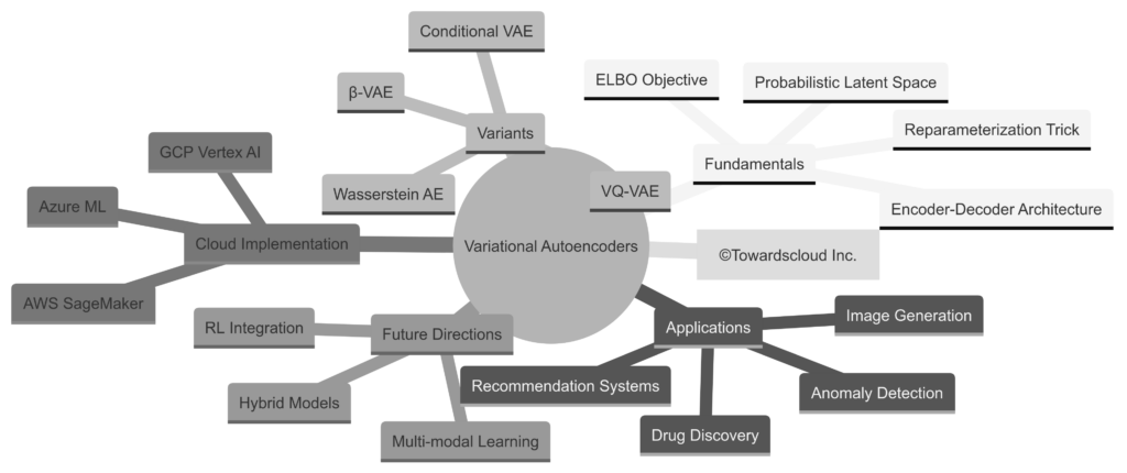
As VAE research has progressed, several advanced variants have emerged to address limitations and enhance capabilities:

1. Conditional VAEs (CVAEs)

CVAEs allow for conditional generation by incorporating label information during both training and generation.

2. β-VAE

β-VAE introduces a hyperparameter β that controls the trade-off between reconstruction quality and latent space disentanglement.

3. VQ-VAE (Vector Quantized-VAE)

VQ-VAE replaces the continuous latent space with a discrete one through vector quantization, enabling more structured representations.

4. WAE (Wasserstein Autoencoder)

WAE uses Wasserstein distance instead of KL divergence, potentially leading to better sample quality.

Advanced VAE Variants Comparison

VAE Variant	Key Innovation	Advantages	Best Use Cases
Conditional VAE (CVAE)	Incorporates label information	Controlled generation, Better quality for labeled data	Image generation with specific attributes, Text generation in specific styles
β-VAE	Weighted KL divergence term	Disentangled latent representations, Control over regularization strength	Feature disentanglement, Interpretable representations
VQ-VAE	Discrete latent space	Sharper reconstructions, Structured latent space	High-resolution image generation, Audio synthesis
WAE	Wasserstein distance metric	Better sample quality, More stable training	High-quality image generation, Complex distribution modeling
InfoVAE	Mutual information maximization	Better latent space utilization, Avoids posterior collapse	Text generation, Feature learning

📚 Call to Action: Which advanced VAE variant interests you the most? Do you have experience implementing any of these? Share your thoughts or questions!

VAEs vs. Other Generative Models

Let’s compare VAEs with other popular generative models to understand their relative strengths and weaknesses:

Generative Models Detailed Comparison

Feature	VAEs	GANs	Diffusion Models	Flow-based Models
Sample Quality	Medium (often blurry)	High (sharp)	Very High	Medium to High
Training Stability	High	Low	High	Medium
Generation Speed	Fast	Fast	Slow (iterative)	Fast
Latent Space	Structured, Continuous	Unstructured	N/A (noise-based)	Invertible
Mode Coverage	Good	Limited (mode collapse)	Very Good	Good
Interpretability	Good	Poor	Medium	Medium

🤔 Call to Action: Based on the comparison above, which generative model seems most suitable for your specific use case? Share your thoughts!

Best Practices for VAE Implementation

When implementing VAEs in production environments, consider these best practices:

1. Architecture Design

• Start with simple architectures and gradually increase complexity
• Use convolutional layers for image data and recurrent layers for sequential data
• Balance the capacity of encoder and decoder networks

2. Training Strategies

• Use annealing for the KL divergence term to prevent posterior collapse
• Monitor both reconstruction loss and KL divergence during training
• Use appropriate learning rate schedules

3. Hyperparameter Tuning

• Latent dimension size significantly impacts generation quality and representation power
• Balance between reconstruction and KL terms (consider β-VAE approach)
• Batch size affects gradient quality and training stability

4. Deployment Considerations

• Convert models to optimized formats (TensorFlow SavedModel, ONNX, TorchScript)
• Consider quantization for faster inference
• Implement proper monitoring for drift detection
• Design with scalability in mind

VAE Implementation Best Practices

Area	Best Practice	AWS Implementation	GCP Implementation	Azure Implementation
Data Storage	Use efficient, cloud-native storage formats	S3 + Parquet/TFRecord	GCS + Parquet/TFRecord	Azure Blob + Parquet/TFRecord
Training Infrastructure	Use specialized hardware for deep learning	EC2 P4d/P3 instances	Cloud TPUs, A2 VMs	NC-series VMs
Model Management	Version control for models and experiments	SageMaker Model Registry	Vertex AI Model Registry	Azure ML Model Registry
Deployment	Scalable, low-latency inference	SageMaker Endpoints, Inferentia	Vertex AI Endpoints	Azure ML Endpoints
Monitoring	Track model performance & data drift	SageMaker Model Monitor	Vertex AI Model Monitoring	Azure ML Data Drift Monitoring
Cost Optimization	Use spot/preemptible instances for training	SageMaker Managed Spot Training	Preemptible VMs	Low-priority VMs

📈 Call to Action: Which of these best practices have you implemented in your ML pipelines? Are there any additional tips you’d recommend for VAE deployment?

Challenges and Limitations of VAEs

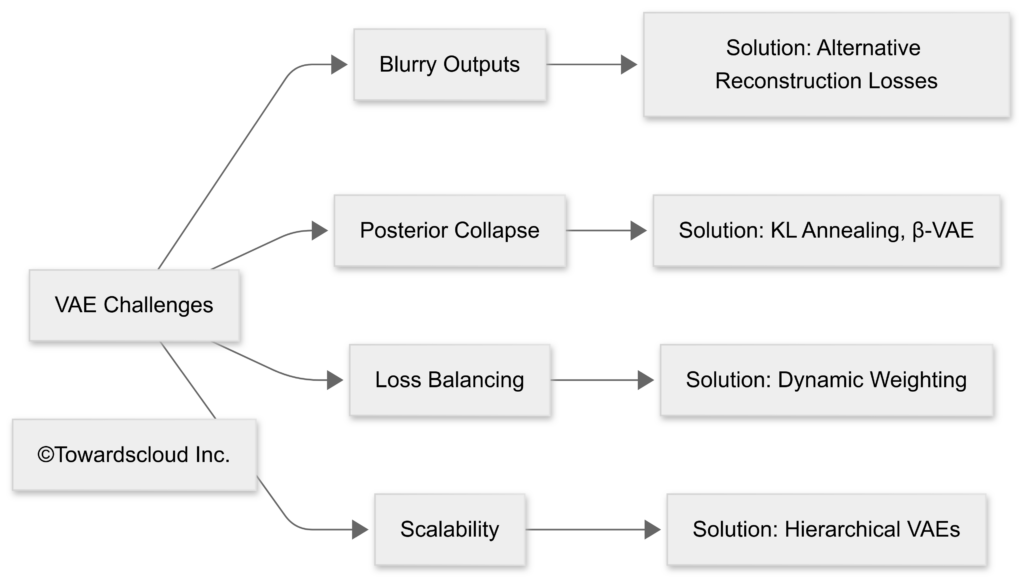
While VAEs offer powerful capabilities, they also come with challenges:

1. Blurry Reconstructions

VAEs often produce blurrier outputs compared to GANs, especially for complex, high-resolution images.

2. Posterior Collapse

In certain scenarios, the model may ignore some latent dimensions, leading to suboptimal representations.

3. Balancing the Loss Terms

Finding the right balance between reconstruction quality and KL regularization can be challenging.

4. Scalability Issues

Scaling VAEs to high-dimensional data can be computationally expensive.

🛠️ Call to Action: Have you encountered any of these challenges when working with VAEs? How did you address them? Share your experiences!

Future Directions for VAE Research

The field of VAEs continues to evolve rapidly. Here are some exciting research directions:

1. Hybrid Models

Combining VAEs with other generative approaches (like GANs or diffusion models) to leverage complementary strengths.

2. Multi-modal VAEs

Developing models that can handle and generate multiple data modalities (e.g., text and images together).

3. Reinforcement Learning Integration

Using VAEs as components in reinforcement learning systems for better state representation and planning.

4. Self-supervised Learning

Integrating VAEs into self-supervised learning frameworks to learn better representations from unlabeled data.

🔮 Call to Action: Which of these future directions excites you the most? Are there other potential applications of VAEs that you’re looking forward to?

Conclusion

Variational Autoencoders represent a powerful framework for generative modeling, combining the strengths of deep learning with principled probabilistic methods. From their fundamental mathematical foundations to their diverse applications across industries, VAEs continue to drive innovation in AI and machine learning.

As cloud platforms like AWS, GCP, and Azure enhance their ML offerings, implementing and deploying VAEs at scale becomes increasingly accessible. Whether you’re interested in generating realistic images, detecting anomalies, or discovering patterns in complex data, VAEs offer a versatile approach worth exploring.

📝 Call to Action: Did you find this guide helpful? What other deep learning topics would you like us to cover in future articles? Let us know in the comments below!

Additional Resources

• Tutorial: VAEs from Scratch with PyTorch – Original VAE paper by Kingma & Welling
• AWS Deep Learning AMIs Documentation
• GCP Vertex AI Documentation
• Azure Machine Learning Documentation
• TensorFlow VAE Tutorial
• PyTorch VAE Examples

We hope this comprehensive guide has given you a solid understanding of Variational Autoencoders and how to implement them on various cloud platforms. Stay tuned for more in-depth articles on advanced machine learning topics!